Most wearables measure HRV (heart rate variability) using one of two formulas, SDNN and RMSSD. But the medical literature has dozens of ways to quantify HRV.

The field of heart rate variability analysis has produced a remarkable zoo of metrics since the 1996 ESC/NASPE Task Force published its foundational standards paper. Each metric extracts different information from the same raw signal: the time intervals between consecutive heartbeats (called R-R or N-N intervals, where “N” means normal, non-ectopic beats).

HRV metrics fall into four broad categories: time-domain, frequency-domain, nonlinear, and time-frequency methods. This post covers all of them. For how specific wearables implement HRV, see our companion post on how different wearables measure HRV.

Time-domain HRV methods

Time-domain metrics are the simplest. They apply basic statistical operations directly to the sequence of N-N intervals or their differences.

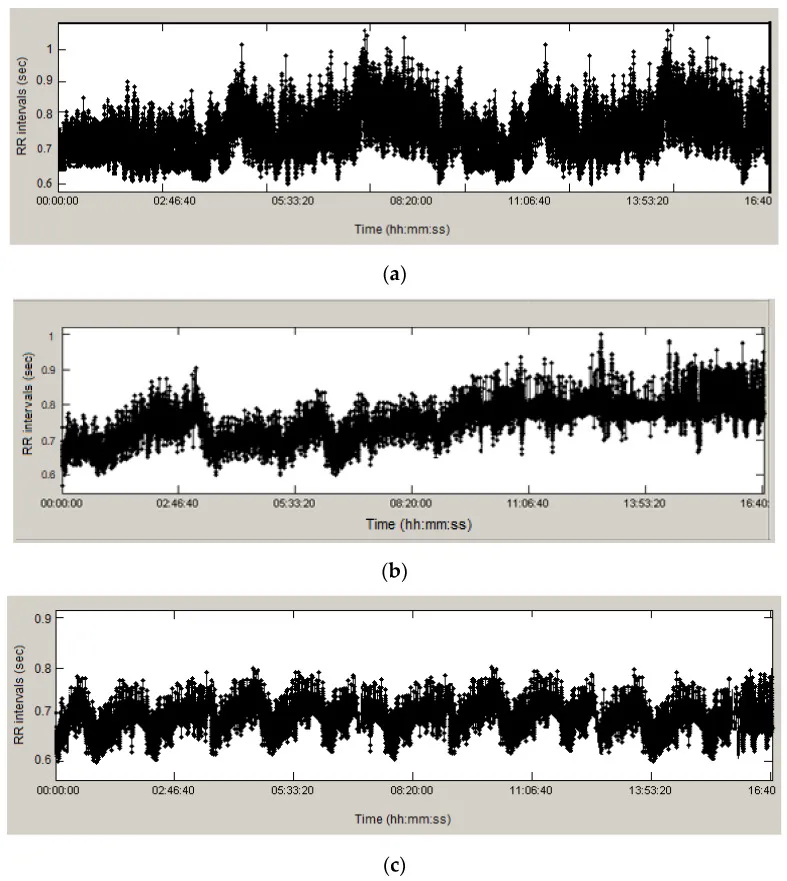RR interval tachograms — the raw input to all HRV analysis — for (a) healthy, (b) arrhythmic, and (c) ischemic patients. Source: PMC10417764, CC-BY 4.0.

SDNN: standard deviation of N-N intervals

The most widely cited HRV metric is SDNN. It’s calculated as the standard deviation of all normal-to-normal beat intervals in a recording window:

SDNN = √[ Σ(NNᵢ - NN̄)² / (N - 1) ]

SDNN reflects total autonomic variability (both sympathetic and parasympathetic branches), plus slower regulatory cycles like circadian rhythm and thermoregulation. SDNN is commonly used for clinical risk stratification from 24-hour Holter recordings.

SDNN is highly dependent on recording duration. A 5-minute SDNN and a 24-hour SDNN are fundamentally different measurements and must never be compared. Longer recordings capture more sources of variability (circadian shifts, activity changes), producing higher values.

Clinical thresholds from 24-hour recordings: SDNN < 50 ms is classified as “unhealthy” and independently predicts post-MI mortality (relative risk ~2.8). SDNN of 50–100 ms indicates compromised health. SDNN > 100 ms is considered healthy. The population mean for healthy adults is approximately 141 ± 39 ms.

SDNN is the metric Apple Watch reports (as heartRateVariabilitySDNN in HealthKit), though Apple Watch measures HRV over ~60-second windows rather than 24 hours.

RMSSD: root mean square of successive differences

RMSSD looks at the difference between each consecutive pair of N-N intervals. Then it squares those differences, averages them, and takes the square root:

RMSSD = √[ Σ(NNᵢ₊₁ - NNᵢ)² / (N - 1) ]

Because RMSSD focuses on beat-to-beat changes, RMSSD is dominated by fast parasympathetic (vagal) activity. It correlates strongly with high-frequency power in the frequency domain (covered below). It’s also less sensitive to recording duration than SDNN, which makes it more reliable for short overnight windows.

The normal range of RMSSD for healthy adults is approximately 19–75 ms. For elite athletes, it’s higher at 35–107 ms. RMSSD is the metric most wearables report, including WHOOP, Oura, Fitbit, Samsung, and Pixel Watch.

SDANN: standard deviation of 5-minute averages

Divide the recording into consecutive 5-minute segments. Compute the mean N-N interval for each segment. SDANN is the standard deviation of those segment means.

This filters out beat-to-beat variation entirely and captures only long-term, slow-cycling variability: circadian rhythms, thermoregulation, hormonal cycles. It requires at least several hours of data and is typically computed from 24-hour Holter recordings.

SDANN is strongly associated with mortality prediction post-MI and correlates with ultra-low frequency power in spectral analysis.

SDNN index (SDNNI)

The complement of SDANN. Divide the 24-hour recording into 288 consecutive 5-minute segments. Compute the standard deviation of N-N intervals within each segment. SDNN index is the mean of those 288 standard deviations.

It captures average short-term variability — cycles shorter than 5 minutes. Together with SDANN, it decomposes total variance: SDNN² ≈ SDANN² + SDNNI².

pNN50 and NN50

NN50 counts the number of consecutive N-N interval pairs where the difference exceeds 50 ms. pNN50 expresses that count as a percentage of total intervals.

pNN50 = NN50 / (N - 1) × 100%

Both reflect parasympathetic activity, similar to RMSSD. However, RMSSD is generally preferred because pNN50 has a more discrete distribution and provides less statistical power. Some researchers use a 20 ms threshold (pNN20) for greater sensitivity in populations with low baseline HRV.

Geometric methods: HRV triangular index and TINN

These methods use the shape of the N-N interval histogram rather than raw statistics.

HRV triangular index (HTI): Construct a histogram of all N-N intervals with a bin width of 1/128 seconds (~7.8 ms). HTI = total number of intervals ÷ the height of the tallest bin. A wider, flatter histogram yields a higher index — more variability.

TINN (Triangular Interpolation of the N-N Interval Histogram): Fit a triangle to the histogram using least-squares minimization. TINN is the baseline width of the best-fit triangle, in milliseconds.

The major advantage of geometric methods is their relative insensitivity to artifact. A few ectopic beats that would corrupt SDNN or RMSSD have less effect on the histogram shape. The 1996 Task Force recommended both for 24-hour recordings.

Less common time-domain metrics

SDSD (Standard Deviation of Successive Differences): Mathematically equivalent to RMSSD for stationary signals, so rarely reported separately.

Baevsky Stress Index: Developed for the Soviet space program. SI = (AMo × 100%) / (2 × Mo × MxDMn), where Mo is the modal R-R interval, AMo is the histogram peak height, and MxDMn is the range. Higher values indicate sympathetic dominance and stress. Normal resting range: 80–150. Now used by Kubios and Garmin.

Deceleration Capacity (DC) and Acceleration Capacity (AC): Computed via Phase-Rectified Signal Averaging (PRSA). DC captures the heart’s ability to slow down (vagal modulation); AC captures its ability to speed up (sympathetic modulation). Bauer et al. (The Lancet, 2006) showed that DC < 4.5 ms was a more powerful predictor of post-MI mortality than LVEF — the existing gold standard.

Frequency-domain HRV methods

Frequency-domain analysis decomposes the N-N interval time series into its wave components using power spectral density (PSD) estimation (e.g., Fourier transforms). The result is a spectrum showing how much power exists at each frequency. This reveals distinct physiological mechanisms operating at different timescales, which is something time-domain metrics can’t disentangle.

How the spectrum is computed

Three main approaches:

FFT (Welch periodogram): The N-N time series is resampled at a uniform rate (typically 4 Hz via cubic spline interpolation), divided into overlapping windows, and transformed via Fast Fourier Transform. Simple and fast, but assumes stationarity within each window.

Autoregressive (AR) modeling: The N-N series is modeled as an autoregressive process (typically using the Burg algorithm). AR methods produce smoother spectra with better frequency resolution on short records, but the model order must be chosen carefully — too low smooths out peaks, too high introduces spurious ones.

Lomb-Scargle periodogram: Works directly on the unevenly spaced R-R intervals without resampling. Avoids interpolation artifacts. Increasingly popular but not yet as widely adopted in clinical literature.

The 1996 Task Force noted that FFT and AR methods yield comparable results in most cases.

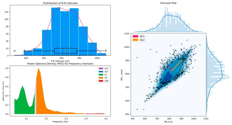Power spectral density of HRV with color-coded frequency bands (ULF, VLF, LF, HF), alongside the RR interval distribution and a Poincaré plot. Source: Pham et al. 2021, Sensors, CC-BY 4.0.

HRV frequency bands

ULF — ultra-low frequency (≤ 0.003 Hz)

Oscillation periods from ~5.5 minutes to 24 hours. Requires a 24-hour recording. Driven by circadian rhythms, core body temperature, the renin-angiotensin-aldosterone system, and metabolic processes. ULF dominates total power in 24-hour recordings. Low ULF has been associated with increased arrhythmic death risk.

VLF: very low frequency (0.003–0.04 Hz)

Oscillation periods of ~25–300 seconds. The most debated band. Shaffer & Ginsberg (2017) identify its primary generator as the heart’s intrinsic cardiac nervous system — the ~40,000 neurons on the heart itself. Parasympathetic blockade almost completely abolishes VLF power, suggesting significant vagal contribution. Additional drivers include thermoregulation and the renin-angiotensin system.

Despite being the least physiologically understood band, VLF is more strongly associated with all-cause mortality than either LF or HF power. Low VLF has been linked to increased inflammation and higher arrhythmic death risk post-MI.

LF: low frequency (0.04–0.15 Hz)

Oscillation periods of ~7–25 seconds. This is where the controversy lives.

The original 1996 Task Force interpretation held that LF reflects both sympathetic and parasympathetic activity. Many researchers simplified this to “LF = sympathetic,” which is now considered incorrect. Evidence from cholinergic blockade studies shows that parasympathetic activity contributes ~50% of LF power, sympathetic ~25%, and other factors (baroreflex mechanics, respiratory crossover) ~25%.

Goldstein et al. (2011) argue that LF power is best understood as an index of baroreflex-mediated cardiac autonomic modulation — the arterial baroreflex’s ability to adjust heart rate in response to blood pressure fluctuations. Key evidence: direct cardiac norepinephrine spillover measurements show no correlation with LF power; heart failure patients have very high sympathetic outflow but very low LF power.

An important confound: slow breathing (below ~8.5 breaths per minute) shifts respiratory sinus arrhythmia into the LF band, artificially inflating LF power. This is why resonance-frequency biofeedback at ~6 bpm produces a massive LF spike at 0.1 Hz.

HF: high frequency (0.15–0.40 Hz)

Oscillation periods of ~2.5–7 seconds, corresponding to breathing at 9–24 breaths per minute. The most straightforward band. HF reflects parasympathetic (vagal) activity driving respiratory sinus arrhythmia (RSA) — heart rate accelerates during inspiration and decelerates during expiration.

HF correlates strongly with RMSSD and pNN50 in the time domain.

Caveat from Shaffer & Ginsberg: HF power does not equal vagal tone. Changes in breathing rate or depth shift HF power without necessarily changing underlying vagal activity. Only under controlled conditions with normal breathing rates (12–20 bpm) can HF approximate vagal tone.

Normal values (5-min supine): ~657 ± 777 ms².

LF/HF ratio

Originally proposed as an index of “sympathovagal balance.” Now widely considered problematic.

Billman (2013) showed that the four assumptions underlying LF/HF are all false: LF is not mainly sympathetic; HF is not exclusively parasympathetic; autonomic responses are not always reciprocal; and sympathetic-parasympathetic interactions are nonlinear. Identical LF/HF values can arise from completely different autonomic states — doubling parasympathetic activity at constant sympathetic levels produces the same ratio as halving sympathetic activity.

Many experts now advise against using LF/HF as a standalone index. If reported, it should be accompanied by absolute LF and HF values.

Normalized units

LF and HF power can be expressed in normalized units: LF(nu) = LF / (LF + HF) and HF(nu) = HF / (LF + HF). These always sum to 1. Quintana & Heathers (2014) showed that LF(nu), HF(nu), and LF/HF are algebraically pairwise redundant — reporting all three is circular.

Normalized units also mask absolute changes. A rise in HF(nu) could mean HF power increased, LF power decreased, or both. Always report absolute power alongside normalized units.

Nonlinear HRV methods

Nonlinear methods capture dynamics (chaos, fractal scaling) that time-domain and frequency-domain metrics miss.

Poincaré plot analysis (SD1, SD2)

Plot each R-R interval against the next one (RR(n) vs RR(n+1)). Fit an ellipse to the scatter cloud.

SD1 (ellipse width, perpendicular to the identity line): measures beat-to-beat variability. Mathematically, SD1 = RMSSD / √2. Reflects parasympathetic modulation.

SD2 (ellipse length, along the identity line): captures longer-term variability. Reflects both sympathetic and parasympathetic influences.

SD1/SD2 ratio: indexes the ratio of short- to long-term variability. The shape of the plot itself is clinically informative: healthy hearts produce a comet shape; heart failure produces a torpedo; atrial fibrillation produces a circular scatter.

Detrended Fluctuation Analysis (DFA α1, α2)

DFA extracts the fractal scaling properties of the R-R time series. The algorithm integrates the series, divides it into windows of varying sizes, fits local trends in each window, and computes the residual fluctuation at each scale. Plotting log(fluctuation) vs log(window size) yields scaling exponents:

• α1 (short-term, windows of 4–11 beats): reflects baroreceptor reflex activity.
• α2 (long-term, windows of 12–64+ beats): reflects slower regulatory mechanisms.

A healthy heart exhibits fractal-like 1/f behavior (α ≈ 1.0). Deviation in either direction — toward 0.5 (white noise, random) or 1.5 (Brownian motion, over-correlated) — indicates disease.

This is arguably the most clinically validated nonlinear HRV metric. In post-MI studies, α1 < 0.85 was the single best univariable predictor of mortality (relative risk 3.17, 95% CI 1.96–5.15) — superior to all traditional HRV measures. In the Cardiovascular Health Study (8-year follow-up, 267 deaths), decreased α1 was the strongest mortality predictor among all HRV measures tested.

Sample Entropy (SampEn)

SampEn quantifies the complexity and unpredictability of the R-R time series. It measures the likelihood that patterns of length m that are similar (within tolerance r) remain similar when extended to length m+1.

SampEn(m, r) = -ln(A / B)

where A = number of template matches of length m+1, and B = number of matches of length m. Standard parameters: m = 2, r = 0.2 × SDNN.

Higher SampEn = more complex, irregular dynamics (generally healthy). Lower SampEn = more regular, predictable signal (often pathological). SampEn was developed to fix biases in the older Approximate Entropy (ApEn) metric, which counted self-matches.

Multiscale Entropy (MSE)

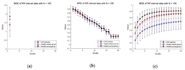Multiscale entropy comparison: CHF patients vs. healthy elderly vs. healthy young subjects. Healthy young subjects maintain higher entropy across scales. Source: PMC7512536, CC-BY 4.0.

MSE evaluates sample entropy across multiple time scales, producing a complexity profile rather than a single number. The R-R series is progressively “coarse-grained” — averaged over windows of increasing size — and SampEn is computed at each scale.

A truly complex system maintains high entropy across many scales. Disease and aging cause entropy to drop at longer scales — the system loses its multi-scale organizational structure. Atrial fibrillation shows a distinctive pattern: high entropy at short scales (randomness) but low entropy at long scales (loss of organized structure).

Correlation Dimension (D2)

Estimates the minimum number of independent variables needed to model the system’s dynamics. Healthy hearts have D2 ≈ 3.3–4.2, reflecting multiple interacting regulatory mechanisms. Disease reduces dimensionality as subsystems fail or decouple. Requires long recordings (1000+ beats).

Lyapunov Exponents

Quantify the rate at which nearby trajectories in the system’s state space diverge — the hallmark of deterministic chaos. Positive exponents indicate chaotic dynamics. The healthy heart exhibits deterministic chaos (λ ≈ 0.25–0.69 bits/beat). Aging and cardiac pathology reduce the Lyapunov exponent, reflecting a paradoxical shift toward more regular but less healthy dynamics.

Symbolic Dynamics

The R-R series is converted into a sequence of symbols (e.g., 0, 1, 2, 3) based on whether intervals are above/below a threshold and increasing/decreasing. “Words” of length 3 are formed and classified:

• 0V words (all symbols identical): low variability, sympathetic dominance
• 2UV/2LV words (all symbols differ): high variability, parasympathetic modulation

Symbolic dynamics enhances risk stratification accuracy above 85% compared to standard HRV measures (Voss et al., Circulation, 2006) and catches cases that traditional HRV classifies as low risk.

Recurrence Quantification Analysis (RQA)

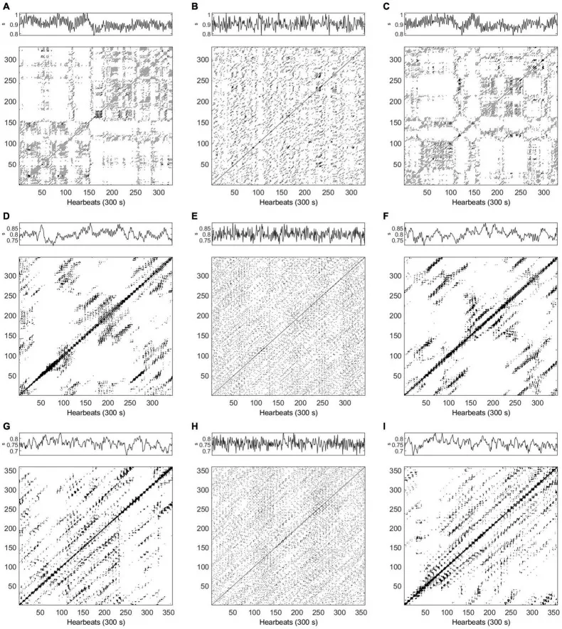Recurrence plots of HRV data in supine position, comparing healthy subjects and ESRD patients. The structure of the plot reveals the system’s deterministic properties. Source: PMC8864246, CC-BY 4.0.

RQA constructs a recurrence plot — a binary matrix showing when the system revisits similar states — and extracts metrics like determinism (percentage of recurrent points forming diagonal lines) and divergence (inverse of the longest diagonal). High determinism indicates stable, predictable dynamics. RQA has achieved 88% accuracy distinguishing coronary heart disease from healthy controls.

Time-frequency methods

Standard frequency-domain analysis gives you one spectrum averaged over the entire recording. Time-frequency methods show how the spectrum evolves over time.

Wavelet analysis

Wavelet transforms decompose the signal using scaled and translated wavelets, providing simultaneous time and frequency localization. Unlike STFT, wavelets use long windows for low frequencies and short windows for high frequencies — ideal for HRV, where LF components evolve slowly and HF components change rapidly.

Wavelet analysis can track acute autonomic responses to tilt-table tests, exercise, mental stress, and sleep stage transitions with higher temporal resolution than FFT. Studies have shown it gives “significantly better quantitative analysis of HRV than Fourier transform during autonomic nervous system adaptations.”

Short-Time Fourier Transform (STFT)

STFT applies the standard Fourier transform to short, overlapping windows, producing a spectrogram. The key limitation vs. wavelets: the window length is fixed, creating a rigid tradeoff between time and frequency resolution.

Summary of all HRV methods

Category	Metric	Primarily reflects	Min recording
Time-domain	SDNN	Total ANS	5 min (short-term); 24h (gold standard)
	RMSSD	Parasympathetic (vagal)	~1 min
	SDANN	Long-term regulation	24h
	SDNN index	Short-term autonomic	24h
	pNN50	Parasympathetic	~2 min
	HTI / TINN	Total HRV (artifact-robust)	24h
	DC / AC	Vagal (DC) / Sympathetic (AC)	5 min
	Stress Index	Sympathetic dominance	2–5 min
Frequency-domain	ULF (≤0.003 Hz)	Circadian, thermoregulation	24h
	VLF (0.003–0.04 Hz)	Intrinsic cardiac neurons, thermoregulation	5 min (24h preferred)
	LF (0.04–0.15 Hz)	Baroreflex modulation (mixed ANS)	2 min
	HF (0.15–0.40 Hz)	Parasympathetic / RSA	1 min
Nonlinear	SD1 / SD2	Vagal (SD1) / mixed (SD2)	5 min
	DFA α1	Fractal scaling (short-term)	~1000 beats
	SampEn	Signal complexity	200+ beats
	MSE	Multi-scale complexity	24h preferred
	Correlation Dimension	System dimensionality	1000+ beats
	Symbolic Dynamics	Sympathovagal patterns	5 min
	RQA	Deterministic structure	5 min
Time-frequency	Wavelet	Time-varying autonomic tracking	Flexible
	STFT	Time-varying spectral analysis	2–5 min

What your wearable gives you vs. HRV methods exists

Consumer wearables report one metric: SDNN (Apple Watch) or RMSSD (everyone else). That’s one row out of the table above. The full landscape of HRV analysis is far richer. That said, the American College of Cardiology advises against interpreting absolute HRV values regardless of which metric you use. The most useful HRV signal (from any device, using any formula) is your personal trend over time.